mean residence time
Mean Residence Time in Flow Reactors: How to Interpret the Average Without Overreading It
Mean residence time is one RTD point, not the full description
Mean residence time is a summary used in local reactor models: it represents one point of the residence-time distribution, while the full distribution may be needed for more accurate conversion and selectivity modeling. You can use the average to compare observed transit behavior with a hydraulic expectation, but the average does not show how widely individual fluid elements differ in their time inside the system.
The central interpretive choice is whether the question can be represented by one RTD point or calls for the full distribution, whose shape may affect conversion and selectivity modeling.
Residence-time-distribution analysis answers a wider question by describing how transit times are distributed across fluid elements. That broader view can help diagnose operating-reactor problems and support modeling of conversion or effluent concentration, but it still does not make an unqualified process decision without the relevant reactor, tracer, and performance context.
What the nominal hydraulic time tells you
Nominal hydraulic residence time is the volume-flow calculation (\tau_h = V_R/Q), where (V_R) is the streamed reactor volume and (Q) is the volumetric flow rate. The calculation gives you a hydraulic benchmark based on the volume and flow values you choose, rather than a direct observation of every fluid element’s path.
A measured mean residence time comes from observed transit behavior, such as time-averaging an outlet pulse response or using the residence-time-distribution density. The nominal hydraulic time comes from bulk volume and flow. Comparing the two is useful because it separates an expected hold-up calculation from the behavior revealed by a tracer response.
The hydraulic comparison becomes meaningful only when the volume, flow rate, and measured path refer to the same process boundary. A stated vessel volume may not represent every active or inactive region that affects transit, and a flow value may not describe the same operating condition as the tracer test. Treat the calculated time as a reference point, not as proof that every part of the process follows that time.
Before comparing a nominal hydraulic time with a measured mean, record:
- the volume included in the calculation;
- the volumetric flow rate and its operating condition;
- the inlet and outlet boundaries used for the measurement; and
- whether the tracer test and the hydraulic calculation represent the same process arrangement.
A comparison with mismatched boundaries can create an apparent deviation that says little about the reactor itself.
How the RTD turns one average into a distribution
Residence time distribution describes how long different fluid elements spend in a reactor or flow system. Instead of assigning one identical time to every element, RTD analysis represents a range of transit times and shows how that range is distributed.
A tracer experiment commonly introduces a tracer at the inlet and measures its concentration at the outlet over time. For a pulse injection, the outlet tracer concentration is proportional to the RTD. The resulting concentration-time response provides the raw pattern from which the mean, spread, and other distribution features can be evaluated.
The mean is one summary extracted from that response. It tells you the distribution’s average time, but it does not tell you whether the response is narrow, broad, skewed, or composed of more than one visible feature. Two systems can therefore share a similar mean while having different transit-time patterns.
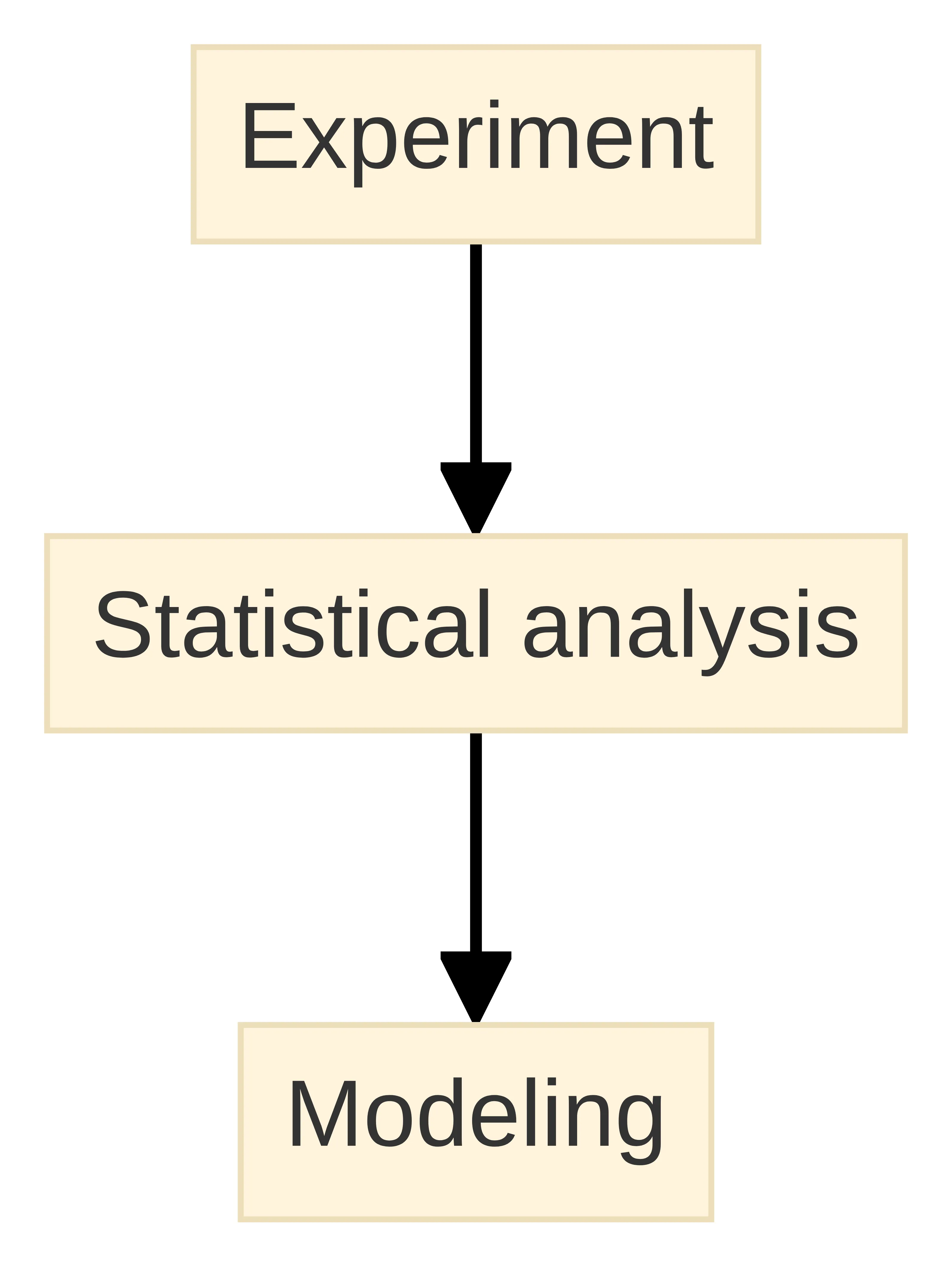
RTD work usually has three linked stages:
- Experiment: introduce a tracer and measure outlet concentration over time.
- Statistical analysis: normalize and examine the response as a distribution.
- Modeling: use the distribution or a suitable representation to investigate the flow system.
The mean belongs inside that sequence. It is not a replacement for the response that produced it.
Normalization provides another reason to retain the distribution rather than only its mean. Dividing each time value by the mean creates dimensionless time, which allows distributions from different systems to be compared on a common relative scale. That comparison can show whether a response is concentrated near its own mean or extends substantially before or after it, even when the systems have different absolute hydraulic times. The comparison remains interpretive rather than a substitute for matching process boundaries: systems must still be described in terms of the inlet, outlet, operating condition, and measurement method that produced each response.
What ideal plug flow and CSTR behavior reveal
Ideal plug-flow and continuously stirred tank reactor behavior provide reference patterns for interpreting an RTD, not universal descriptions of real equipment. Plug flow assigns the same residence time to all molecules in the idealized comparison, while a CSTR produces a broad range that includes very short exit times.
| Reference behavior | Residence-time pattern | What the comparison helps you ask |
|---|---|---|
| Ideal plug flow | All molecules are described as spending the same time in the reactor. | Is the measured distribution narrow relative to the ideal reference? |
| Ideal CSTR | Material is completely mixed, with a broad residence-time range that includes very short exit times. | Does the measured response show the broad behavior expected from extensive mixing? |
| Real flow system | Channeling, stagnant regions, bypassing, longitudinal mixing, turbulence, or imperfect mixing can spread the times. | Which nonideal features could explain the observed shape? |
A series of idealized CSTRs also illustrates why reactor arrangement matters. When total volume remains constant, increasing the number of CSTRs in series makes the RTD approach plug-flow behavior. That comparison changes the distribution pattern without changing the total volume, so the mean alone cannot identify the arrangement.
Real unit operations can be represented with combinations of idealized elements, including effects associated with dead zones, nonideal back-mixing, and bypassing. Use the ideal references to frame a question about the measured distribution; do not use them to label a real reactor without examining the actual response.
How a flow-process measurement produces the mean
A flow-process measurement produces a mean by tracking how a tracer signal moves from inlet to outlet. You introduce a known tracer pattern, record the outlet concentration as time passes, and treat the resulting response as information about the residence-time distribution.
A pulse response is especially direct for this purpose: the outlet concentration varies with time, and its time-averaged response or associated distribution density can be used to obtain the mean residence time. The calculation should preserve the time origin, the concentration response, and the process boundary used for the test. Because the outlet pulse concentration is proportional to the RTD, the response carries more information than the final average. Time-averaging gives greater influence to signal located at later times than to an equal amount of signal located earlier, so an extended late response can shift the mean even if the central part of the curve is unchanged. Conversely, an early response component can lower the average. This is why the time origin, response capture interval, and treatment of the concentration signal matter: changing them can change the summary without changing the equipment. A reported mean should remain linked to the response used to calculate it, rather than being treated as an independent property of the reactor.
A measured mean is therefore conditional on the test arrangement. Inlet location, outlet location, flow condition, active volume, tracer behavior, and the interval over which the response is captured all affect what the reported average represents. If those conditions differ from the hydraulic calculation, compare the conditions before interpreting the numerical difference.
Use the measurement record to answer three practical questions:
- What tracer input was applied?
- What outlet concentration response was recorded over time?
- What statistical treatment converted that response into a distribution and mean?
A mean without this context is difficult to connect to a specific flow path or process question. Preserving those details also supports later comparison: if two reported means come from different boundaries, operating conditions, tracer inputs, or capture intervals, describe them as different measurement contexts rather than as direct evidence of a process change.
What a shorter-than-expected mean may indicate
A shorter measured mean than the nominal hydraulic time may indicate that part of the material reaches the outlet sooner than the volume-flow calculation suggests. More generally, real reactors can exhibit bypassing, short-circuiting, or channeling, producing a spread of residence times.
A shorter mean does not identify one mechanism by itself. Bypassing through a connected unit operation, nonuniform flow through a packed region, or a process boundary that excludes part of the intended hold-up can produce different interpretations. Treat the mean as a prompt to inspect the distribution and the test boundary rather than as proof of a specific fault.
When the measured mean is materially shorter, compare:
- the volume and flow values used for the hydraulic calculation;
- the inlet and outlet locations used during the tracer test;
- the early part of the outlet response for a rapid component; and
- the full response for evidence of a later component that the mean may conceal.
These checks distinguish a genuine transit-time difference from a mismatch between the calculation and the experiment.
The direct next action is to inspect the complete tracer response before concluding that the process has a short effective residence time. If the response contains an early feature or a broad tail, report those features with the mean instead of compressing them into one number.
What a longer-than-expected mean may indicate
A longer measured mean than the nominal hydraulic time may indicate that some fluid elements remain in the system longer than the bulk volume-flow calculation suggests. Stagnant regions, dead zones, back-mixing, or other nonideal flow features can extend the observed residence-time pattern.
A longer mean still does not identify a single cause. The assumed volume may not match the active path, the operating flow may differ from the value used in the calculation, or a connected region may contribute a slow response. RTD models use combinations of idealized elements to represent effects such as dead zones and nonideal back-mixing, but selecting a model requires the measured response and process context.
For a longer-than-expected mean, examine:
- the late portion of the outlet response;
- the amount of tracer accounted for in the measurement;
- the volume and flow values used as the hydraulic reference; and
- whether the measured path includes regions that the nominal calculation leaves out.
A long tail can raise the average even when much of the response arrives earlier, so the mean should be read alongside the distribution.
The direct next action is to test whether the longer mean is associated with a tail or a distinct slow feature. If it is, investigate the relevant flow region or unit operation rather than treating the average as a complete description of the process.
Why the mean cannot establish reactor performance
Mean residence time also cannot establish mixing quality. RTD is a characteristic of the mixing that occurs in a reactor, but the average does not show the distribution’s width, early departures, late material, or multiple flow populations. A short mixing time can coexist with dead zones that RTD analysis reveals.
The average cannot establish conversion, selectivity, product distribution, yield, or an acceptable operating condition on its own. Different residence times create different reaction times, and RTD can affect product distribution in polymerization reactors. The process outcome still depends on the reaction and the way the flow distribution interacts with it.
Use the mean to ask whether further analysis is warranted, not to close the performance question. If your decision concerns conversion, effluent concentration, selectivity, product distribution, or process consistency, connect the RTD or another suitable measurement to that specific outcome before drawing a conclusion.
Read spread, tails, and multiple features beyond the mean
The spread of residence times is a separate result from the mean. Variance, also called the second central moment, quantifies that spread. A narrow distribution and a broad distribution can have the same mean, but they imply different levels of transit-time variation. Variance should likewise be treated as a descriptor rather than a diagnosis. It identifies the amount of spread but not where that spread occurs. The same variance could arise from an early and late pair of features, a single broad response, or a skewed tail; the curve is needed to distinguish those possibilities. Thus, report variance with the mean and visible response shape when the purpose is troubleshooting. If a model uses only moments, state that choice because it compresses the measured response and may omit features relevant to a reaction or unit-operation explanation.
The shape of the response can also carry process information. An early feature may be consistent with bypassing or short-circuiting, while a delayed feature or extended tail may be consistent with stagnant regions or dead zones. Those interpretations remain hypotheses until the response, equipment arrangement, and test boundary support them.
Read an RTD result in layers:
- Location: the mean or another central-time measure.
- Spread: variance or a related measure of how widely times are distributed.
- Shape: skew, early response, late tail, or more than one feature.
- Boundary: the part of the process represented by the tracer path.
This layered reading keeps the average useful without allowing it to erase the pattern around it.
A model that uses only the mean is a compact representation. A model that uses the full RTD can represent more of the nonideal behavior relevant to conversion and selectivity. Choose between those levels according to the process question and the features visible in the measured response. That distinction also matters when a model is compared with data. A model can reproduce the central time while missing an early response, a delayed tail, or a second feature. Agreement on the mean therefore does not establish agreement on the flow pattern. When model results are used to explore conversion or selectivity, compare the modeled response with the available distribution features and state whether the model uses the full RTD or only its mean. The more compressed representation may be adequate for a narrowly defined transit question, but it should not be treated as interchangeable with a distribution-based description.
Why mixing time and RTD answer different questions
Mixing time measures how quickly a perturbation homogenizes within a vessel, whereas RTD measures the distribution of fluid-element ages leaving the vessel. The measurements are complementary because one describes an internal homogenization rate and the other describes outlet transit behavior.
A short mixing time does not rule out dead zones. Material can appear well homogenized at a monitored location while some regions contribute delayed fluid to the outlet. RTD analysis can expose that delayed behavior even when a mixing-time result appears favorable.
Use mixing time when your question concerns how quickly a disturbance becomes homogeneous inside the vessel. Use RTD when your question concerns how long fluid elements remain in the system or whether the outlet receives early and late populations. If both internal blending and outlet transit matter, plan the measurements as complementary rather than substituting one for the other.
When the full RTD deserves closer analysis
The full RTD deserves closer analysis when the process question depends on more than an average transit time. That condition applies when the distribution may affect conversion or selectivity, when the measured mean differs materially from the hydraulic reference, or when early and late response features could change how the unit operation is understood.
RTD analysis can help diagnose problems in an operating reactor and can support prediction of conversion or effluent concentrations when a new reaction is used in an existing reactor. Model combinations of idealized elements can also represent dead zones, nonideal back-mixing, and bypassing in real unit operations. One way to connect the curve to a reaction question is the segregated-fluid view used in RTD modeling. Under that framework, fluid elements are treated as small batch reactors that do not mix with one another until they leave the system; each portion’s residence time then supplies its reaction time. The RTD supplies the collection of these times, so a model can evaluate how the range of times, not only its average, contributes to an outlet result. This is a modeling framework, not a claim that every reactor behaves as isolated portions. Its value is diagnostic: it makes explicit why replacing the curve with its mean can remove information needed when reaction behavior varies with residence time. If the question is only where tracer appears, this extra reaction model may be unnecessary; if the question concerns conversion or effluent concentration, the reaction representation and the RTD need to be considered together.
Escalate from the mean to the full distribution when you need to know:
- whether a rapid outlet response precedes the main response;
- whether a delayed tail or separate slow feature exists;
- how much residence-time spread the system has;
- whether the measured pattern changes between operating conditions; or
- whether a model based on the mean would hide a feature relevant to the process outcome.
The practical boundary is simple: a single mean is sufficient only for a question that genuinely requires a single average.
When any of these questions matters, retain and review the concentration-time response rather than reporting only the mean. Use the distribution to decide whether a simple summary remains adequate or whether a fuller model and process-specific measurement are needed.
Which complementary measurements answer the process question
A tracer-based RTD measurement answers the transit question: how are fluid-element residence times distributed between the selected inlet and outlet? The mean and variance summarize that response, while the complete curve preserves early, central, and delayed behavior.
A mixing-time measurement answers a different internal question: how quickly does a perturbation homogenize within the vessel? Use it when internal blending is the concern, and pair it with RTD when outlet age distribution or dead zones also matter.
An outlet concentration or conversion measurement answers the process-outcome question more directly than residence time alone. RTD can support prediction of conversion or effluent concentration, but the relevant outcome still has to be measured or modeled for the reaction and operating condition under consideration.
Match the measurement to the decision:
- Transit behavior: use the tracer response and RTD.
- Internal homogenization: use mixing time.
- Reaction or outlet outcome: use the relevant concentration, conversion, or selectivity measurement, with RTD as supporting flow information.
- Model adequacy: compare a mean-based representation with the full RTD when distribution shape may affect the result.
No single measurement answers all four questions. Separate the evidence needed for a flow diagnosis from the evidence needed for an outcome claim. An early response, late tail, or broad variance can justify investigating nonideal transit, but it does not by itself establish the magnitude of a conversion or selectivity effect. For that second question, preserve the RTD and pair it with the relevant reaction or outlet measurement, or with a model whose assumptions are stated. This distinction prevents a useful diagnostic curve from being overread as a performance result. It also clarifies what to retain in a record: the tracer response for transit interpretation, the chosen spread or shape descriptors for diagnosing nonideal flow, and the process outcome measurement when the decision concerns reaction behavior.
A bounded sequence for interpreting a measured mean
Start with the hydraulic reference. Calculate the volume-flow time from the reactor volume and volumetric flow rate that represent the intended process boundary. Record the values and operating condition instead of treating an unlabeled nominal time as self-explanatory.
Next, define the measured mean. State whether it came from an outlet pulse response or from the residence-time-distribution density, and identify the inlet, outlet, tracer input, and time interval represented by the test.
Then compare like with like. A difference between the measured mean and the hydraulic reference deserves interpretation only after you confirm that volume, flow, process boundary, and operating condition correspond. A boundary mismatch can look like a flow anomaly.
After that, inspect the response shape. Look for an early feature, a broad response, a delayed tail, or multiple features that could be consistent with bypassing, channeling, stagnant regions, dead zones, or nonideal back-mixing. Keep each interpretation conditional until the equipment arrangement supports it.
Add spread and process relevance. Use variance or another supported spread measure to describe how widely residence times vary, then ask whether that variation could affect the conversion, selectivity, effluent concentration, or other outcome under consideration. The mean alone cannot answer that question.
Choose the next measurement. Use mixing time for internal homogenization, the full RTD for transit-time structure, and an outcome measurement for conversion or effluent behavior. Use more than one when the process decision depends on more than one physical question.
End the interpretation at the evidence boundary. A measured mean can indicate that further investigation is warranted, but it cannot establish that a reactor is acceptable, that a process will achieve a particular result, or that one explanation for the deviation is correct without the relevant process conditions and measurements.
What the outlet response can and cannot tell you
Interpret the outlet response by its features: an early portion can raise a question about bypassing or short-circuiting, while a broad or delayed portion can prompt examination of stagnant regions or longitudinal mixing. These are hypotheses about flow behavior, not evidence of a particular conversion, yield, or reactor result.
If your result is difficult to interpret, organize the unresolved question before choosing the next test: transit-time structure, internal homogenization, or reaction outcome. A qualified process or engineering professional should determine individual suitability for a specific reactor, process, or operating decision.