Mean Residence Time: How to Interpret the Average Alongside the Full RTD

Mean residence time answers an average-time question

Mean residence time answers an average-time question: how long, on average, do fluid elements remain inside a reactor or process system? Residence time is the time a fluid element spends within the system boundaries, from entry to departure. The mean combines the residence times of the fluid elements leaving the system into a single time value.

That average is useful, but it is not a complete description of flow. Fluid elements in a real reactor can spend different amounts of time inside the equipment, so the system has a residence-time distribution (RTD) rather than one residence time shared by every element. The mean gives you the distribution’s weighted center; the RTD shows how widely the individual times are spread around it.

For process and reactor analysis, interpret the average through three linked questions:

• What time does the reactor volume and flow rate imply?
• What time does the outlet response actually show?
• What does the full RTD reveal that the average conceals?

The first question establishes a hydraulic reference. The second gives you a measured result. The third determines whether that result is enough for the process decision you need to make.

The nominal expectation comes from volume and flow

A nominal residence-time expectation comes from the reactor volume divided by the volumetric flow rate:

τₙ = V / Q

Here, V is the streamed or reactor volume and Q is the volumetric flow rate. The quotient has units of time. If you use litres for volume and litres per minute for flow, the result is in minutes; the same unit relationship applies with other consistent units. This calculation is also referred to as hydraulic residence time.

Treat V/Q as a baseline for comparison, not as proof that every fluid element experiences that time. The calculation describes what the stated volume and flow would imply under the chosen system boundaries. It does not describe the spread of times created by the way fluid actually moves through the equipment.

Before comparing this baseline with an outlet measurement, define the basis clearly:

• State which equipment and connecting volume are included in V.
• Use the volumetric flow rate that applies to the same system and operating condition.
• Keep the time and volume units consistent.
• Record whether the measured response represents the whole flow path or only a sampled path.

This discipline prevents an accounting difference from being mistaken for a flow difference. A change in volume or flow changes the nominal expectation directly; a difference between that expectation and the measured average requires a separate interpretation.

Measure the average from the outlet response

An outlet tracer experiment gives you a second route to the average. A typical RTD experiment introduces a tracer into the system and measures its concentration as a function of time while the tracer travels through the equipment and exits. The resulting concentration–time response is then normalized for residence-time analysis.

Let C(t) represent the measured tracer concentration at time t. After normalization, the residence-time-distribution density E(t) describes the fraction of outflow whose residence time falls between t and t + dt. The weighted average is calculated as:

τ̄ = ∫ tE(t)dt / ∫ E(t)dt

When E(t) has already been normalized so that its integral is one, this reduces to τ̄ = ∫ tE(t)dt. The same calculation can be applied to discrete or binned data by replacing the integrals with weighted sums:

τ̄ = Σ(tᵢEᵢΔtᵢ) / Σ(EᵢΔtᵢ)

This expression gives each time interval a weight based on the tracer fraction associated with that interval. A small response at a particular time contributes less than a large response at that time.

Use the following sequence when working from measured data:

1. Record the outlet concentration against time from tracer introduction through the relevant exit response.
2. Establish the time intervals represented by the measurements.
3. Normalize the response, or retain the denominator in the weighted-sum equation.
4. Multiply each time value by its normalized response contribution.
5. Sum the weighted contributions and divide by the total response if normalization was not already applied.
6. Compare the resulting average with V/Q calculated on the same system boundary.

The measurement window matters. The outlet pulse response is measured as the tracer exits the apparatus, so truncating the response before the relevant material has left can change the calculated average.

Read mean residence time as the center of the RTD

The RTD is the map of residence times; the mean is its weighted center. In the density notation, E(t)dt represents the fraction of outflow that has resided in the system between t and t + dt. Because E(t) distributes outflow across time, its weighted average incorporates both earlier and later departures.

This distinction lets you interpret the average without treating it as a typical time for every fluid element. A distribution can place some outflow before the mean and some after it. The mean remains mathematically valid even when the response is spread across a wide time range.

You can also put different RTDs on a common time basis by using dimensionless time:

θ = t / τ̄

The current time is divided by the mean, allowing distributions from different systems or operating conditions to be compared after their time scales have been normalized. This comparison changes the time axis; it does not remove differences in the distributions themselves.

RTD analysis uses functions such as E(t) and F(t) to describe flow patterns and departures from ideal plug-flow and perfectly mixed-flow behavior. The practical implication is straightforward: report the mean with the response from which it was calculated. A time value without its distribution leaves you unable to see whether the outflow is concentrated near the center or distributed across substantially earlier and later times.

Compare the measured mean with the nominal baseline

Compare the outlet-derived average with V/Q only after the two values use the same boundaries, volume basis, flow basis, and time units. The comparison asks whether the observed hydraulic average agrees with the volume-to-flow expectation. It does not, by itself, establish ideal flow or process performance.

Bypassing and short-circuiting are recognized causes of nonideal reactor behavior.

Stagnant regions, longitudinal mixing, and imperfect mixing are among the reported causes of departures from ideal flow.

These interpretations are diagnostic possibilities, not automatic findings. The same difference can also result from a mismatched system boundary, an incorrect volume estimate, a flow rate that does not represent the measured period, or a tracer response that does not represent the full stream. Resolve those definitions before assigning a physical explanation.

Use the comparison as a decision point:

• If the average and V/Q are close, continue to the full RTD rather than declaring the reactor ideal.
• If the average is shorter, look for evidence of early arrival, bypassing, short-circuiting, or a nonparticipating volume.
• If the average is longer, look for evidence of delayed material, stagnant regions, or other nonideal flow.
• If the basis is uncertain, correct the measurement and volume–flow definitions before diagnosing the reactor.

Investigate what the average may be hiding

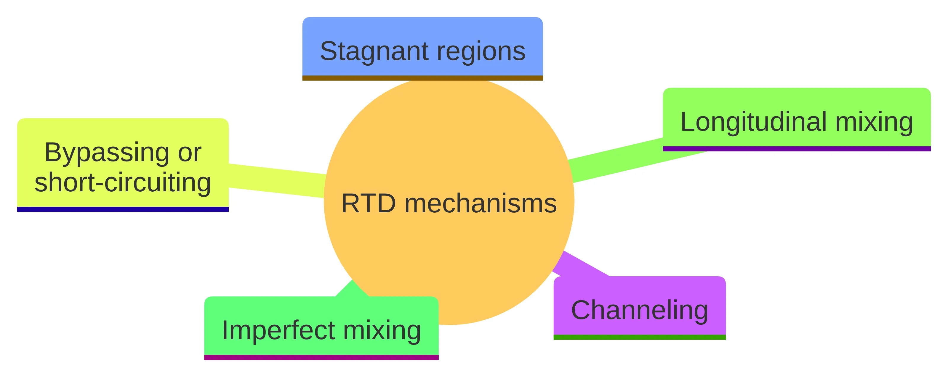
A single average can conceal the flow mechanisms that created it. Real reactors can depart from idealized behavior through several pathways:

• Channeling: part of the fluid follows a preferential route through the system.
• Stagnant regions: some volume contributes differently from the actively flowing region.
• Bypassing or short-circuiting: part of the flow reaches the outlet without experiencing the intended path.
• Longitudinal mixing: material spreads along the flow direction rather than moving with one uniform residence time.
• Imperfect mixing: mixing equipment does not produce the idealized distribution assumed in a simplified model.

These mechanisms can produce a spread of residence times. The RTD records that spread, while the mean compresses it into one value. A shorter portion and a longer portion can therefore coexist in the same response without being visible in the average alone.

To investigate the hidden behavior, examine the outlet concentration–time response and its normalized E(t) representation together. Look for the timing of the first response, the concentration across the main response, and material arriving later than the central part of the response. Then relate those features to the physical flow path and the system boundary.

Do not assign a mechanism from the curve shape alone. Channeling, stagnant regions, bypassing, longitudinal mixing, and imperfect mixing can all produce nonideal behavior, so the response identifies a flow question rather than naming a single cause. RTD analysis is used to diagnose problems in operating reactors, but diagnosis requires the distribution and the relevant equipment context, not merely its mean.

Equal means do not imply equal reactor behavior

Two reactors or operating conditions can have the same average while having different RTD shapes. One response may be concentrated around its center. Another may contain a wider mixture of early and late residence times whose weighted average happens to be the same. The equal averages do not make the two flow patterns interchangeable.

That difference matters whenever material has time-dependent behavior inside the reactor. A mean-only model uses one point of the RTD. Relying on the mean can bias analyses of conversion and selectivity when the distribution materially affects the result; incorporating the entire RTD provides a more detailed alternative.

Match the amount of RTD information to the question you are asking:

• For a hydraulic summary, report the measured average, V/Q, and the system boundaries used for both.
• For flow diagnosis, retain the concentration–time response and inspect the RTD functions rather than reporting only the average.
• For analysis involving conversion or selectivity, use the full RTD when the residence-time spread affects the model.
• For comparison between systems, use dimensionless time as well as the original time scale so that both distribution shape and absolute timing remain visible.

RTD analysis is therefore more than a way to calculate an average. It supplies the information needed to distinguish a compact response from a dispersed one and to evaluate how nonideal flow may influence reactor analysis.

Use the complete RTD before making a process judgment

Use this sequence to interpret an average without losing the flow information around it:

1. Define the system. Specify the reactor or process boundaries, the volume included, and the flow basis.
2. Calculate the hydraulic reference. Use V/Q to establish the nominal time for that defined volume and volumetric flow rate.
3. Determine the measured average. Calculate the weighted average from the normalized outlet response or from E(t).
4. Compare like with like. Check whether the measured and nominal values use the same units, boundaries, operating basis, and response path.
5. Inspect the distribution. Examine E(t), F(t), and the concentration–time response for the spread of residence times and for earlier or later portions that the average cannot show.
6. Choose the right analysis. Use the average for the hydraulic summary, but retain the complete RTD when diagnosing nonideal flow or evaluating conversion and selectivity.

The central conclusion is narrow but useful: the average tells you how residence time is centered, while the full RTD tells you how residence time is distributed. A qualified process professional should decide how those results apply to a specific reactor, process, safety question, or regulatory context.

What should you check when mean residence time and nominal residence time differ?

What is mean residence time in chemical processes?

This metric is the average time that fluid elements spend inside a reactor or process system, calculated as the reactor volume divided by the volumetric flow rate.

How is the average residence time determined from tracer experiments?

It can be determined by conducting a tracer experiment, where a tracer is injected into the system, and its concentration is measured over time. The resulting data is used to calculate the weighted average of residence times.

What can a shorter or longer measured average residence time indicate about reactor flow?

A shorter measured average may suggest that some fluid has taken a shorter path through the reactor, indicating potential bypassing or short-circuiting.

Why should the average residence time not be used alone to characterize a reactor?

The average alone does not provide a complete picture of reactor behavior, as it does not account for the spread of residence times or the shape of the residence time distribution (RTD), which can reveal important flow characteristics.

What is the relationship between the average residence time and the residence time distribution?

This metric is a single value that represents the weighted center of the residence time distribution (RTD), which shows how fluid elements spend varying amounts of time in the reactor.

What are the limitations of using the average residence time in reactor analysis?

Using the average alone can lead to misinterpretations of reactor performance, as it does not capture the full range of residence times or the effects of nonideal flow patterns.