mean residence time
What Is Mean Residence Time? How to Interpret It in Flow Systems
Mean residence time answers one timing question
Mean residence time answers a timing question: how long does material spend in a flow system on average? That answer is useful, but it is not a complete diagnosis of the reactor or process. Real systems can contain a range of passage times because of channeling, stagnant regions, bypassing, longitudinal mixing, turbulence, or imperfect mixing. The average compresses that range into one value. It does not show how the individual times are distributed.
You can establish an initial expectation from the streamed volume and volumetric flow rate, then compare that expectation with a value estimated from tracer-response data. The volume-and-flow calculation gives you a nominal reference for the operating condition. The measured response tells you how the system actually distributed transit times during the test. Treating those as related but distinct quantities prevents a common interpretation error: accepting agreement or disagreement with the average as proof of a specific flow pattern.
The practical sequence is straightforward:
- Define the system boundary and the stream being evaluated.
- Calculate the volume-and-flow expectation.
- Measure or obtain the outlet response from a suitable residence-time-distribution test.
- Estimate the mean from the response.
- Examine the distribution, its spread, and any early or delayed features before drawing a process conclusion.
That sequence keeps the average in its proper role. It is a summary of passage time and a useful comparison point, while the full distribution supplies the context needed to interpret flow behavior.
What mean residence time, nominal time, and RTD each describe
Mean residence time, nominal residence time, and residence time distribution describe different views of the same passage problem. Keeping the terms separate makes your interpretation more precise.
Mean residence time is an average passage time. For a system with streamed volume V and volumetric flow rate Q, the hydraulic mean is defined by the volume divided by the flow rate:
τ = V / Q
This calculation uses the stated or measured operating quantities. It does not require a tracer response, although a response can provide another way to estimate the mean.
Nominal residence time is a practical reference label for the volume-and-flow expectation established before you interpret measured tracer data. In this guide, use it for the value calculated from the specified system volume and flow rate. The distinction is functional rather than diagnostic: nominal time is an expectation based on operating quantities, whereas the measured mean is estimated from how tracer material exits the system. If the two differ, the difference is a reason to inspect the test conditions and the distribution, not a diagnosis by itself.
Residence time distribution, or RTD, describes the range and relative pattern of passage times. A typical experiment introduces a tracer and records its concentration at the outlet over time. After normalization, the outlet response to an instantaneous pulse can be represented as the exit-age distribution E(t), a probability density for the time at which material entering at the initial moment exits the system.
These terms therefore answer different questions:
- Nominal time: what passage time does the specified volume and flow imply?
- Mean: what is the average passage time represented by the measured distribution?
- RTD: how are passage times spread and shaped across the system?
A single mean can agree with the nominal calculation while the distribution still contains important early and late behavior. Conversely, a difference between nominal and measured means tells you that the observed response deserves examination, but it does not identify the cause without the rest of the RTD and the process context.
Use volume and flow to establish the initial expectation
Volume and flow establish the first expectation for passage time. The hydraulic calculation divides the streamed volume in the apparatus by its volumetric flow rate. In compact form:
τV = V / Q
Here, V must represent the volume within the boundary you are analyzing, and Q must represent the corresponding volumetric flow rate. If you calculate the value for a vessel but use a flow rate measured at a different boundary or operating condition, the comparison can lose its meaning. Define the boundary before doing the arithmetic.
Use this calculation as an initial reference, not as a description of every material element. It summarizes the relationship between the stated volume and flow. A real system may give different elements different passage times, and the resulting RTD may show a spread around the average. The volume-and-flow value therefore gives you a baseline against which the measured response can be examined.
Before comparing the calculated value with a tracer result, record:
- The equipment and stream boundary included in V.
- The flow rate and units used for Q.
- The operating condition represented by both quantities.
- Any recirculation or connected volume included in the measurement path.
- Whether the comparison concerns the same configuration and state.
This record does not explain the flow by itself. It makes the reference reproducible and gives you a clear starting point for the RTD interpretation.
Estimate the mean from tracer-response data
Tracer-response data estimate the mean from what exits the system over time. In a typical RTD experiment, you introduce a known tracer input and record the outlet concentration as a function of time. The outlet curve is then normalized so that its area represents the tracer response across the observation period.
At a general level, the calculated mean is the time-weighted average of the normalized residence-time density. Times at which more tracer appears contribute more heavily to the average than times with little tracer. The result can also be obtained by time-averaging the outlet pulse response. Both approaches connect the mean to the observed response rather than to the nominal volume-and-flow expectation alone.
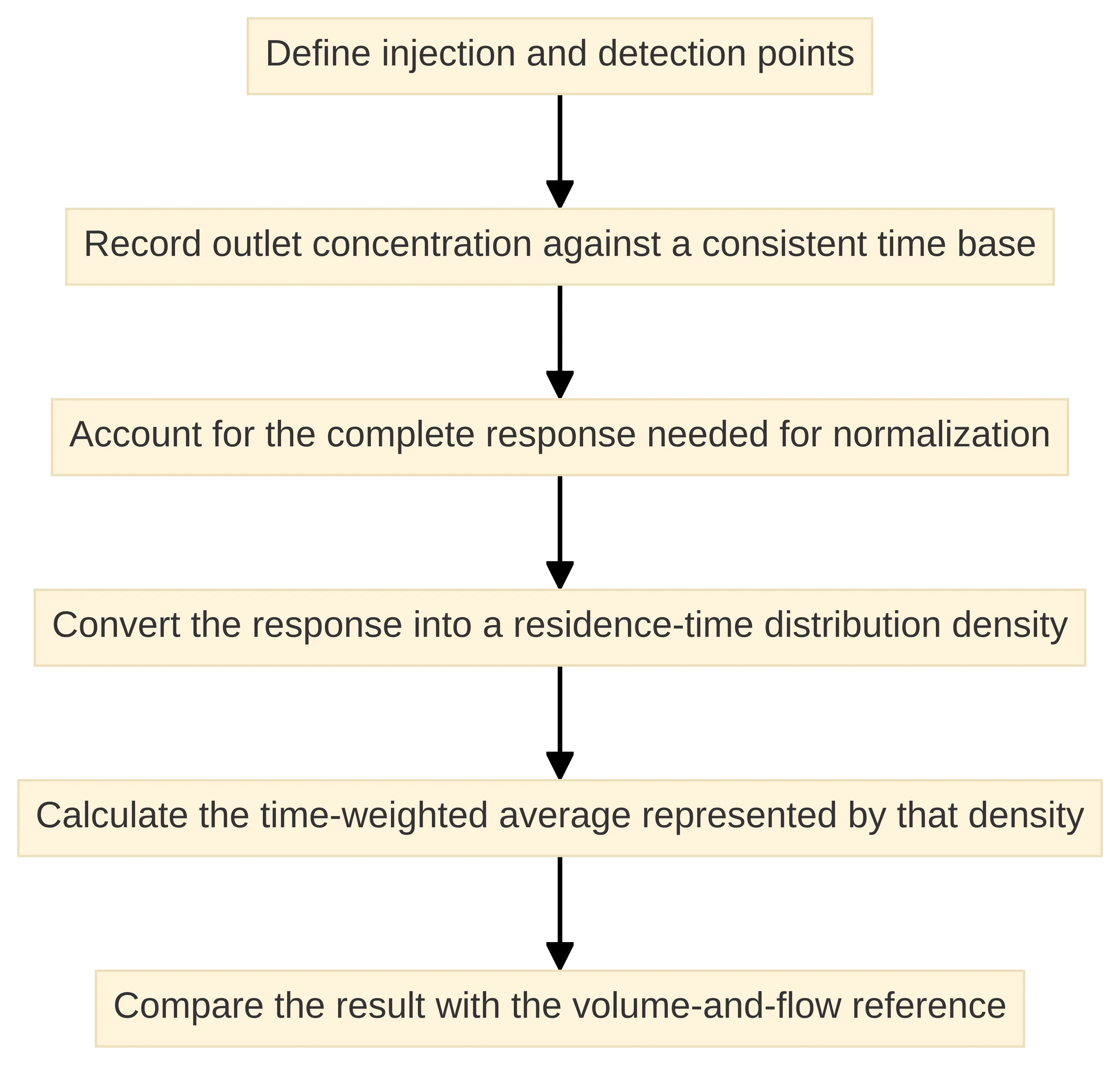
A useful calculation sequence is:
- Define the injection and detection points.
- Record outlet concentration against a consistent time base.
- Account for the complete response needed for normalization.
- Convert the response into a residence-time distribution density.
- Calculate the time-weighted average represented by that density.
- Compare the result with the volume-and-flow reference using the same system boundary.
The injection and detection arrangement matters because the measured distribution describes the path between those locations. A tracer added upstream of a vessel and detected downstream of a connected line characterizes that combined path unless the line is treated separately.
The output of this step is still a summary. It gives you an average passage time derived from the experiment, while the time-by-time response retains information about early arrivals, delayed material, and the width of the distribution. Preserve that response instead of keeping only the single mean.
Read the full residence-time distribution behind the average
The full residence-time distribution shows what the average hides. A real reactor can produce a spread of passage times rather than moving every fluid element through the system at one identical rate. Channeling, stagnant regions, bypassing or short-circuiting, longitudinal mixing, turbulence, and imperfect mixing are among the factors associated with departures from ideal flow behavior.
Read the RTD as a response over time, not as a single point. Start with four questions:
- When does the response begin?
- Where is the main concentration of the response?
- How broadly is the response distributed?
- Does a delayed tail continue after the main response?
An early response can draw attention to short transit paths. A broad or delayed response can draw attention to slower paths or extended residence within the system. These observations are signals for further interpretation, not proof of a particular internal structure. The same mean may arise from different distributions, so the average cannot distinguish among all possible flow patterns.
RTD measurements can reveal transit times, short-circuiting, recirculation zones, and dead zones. They can also support development and validation of flow models. That makes the distribution useful both for direct comparison between operating conditions and for deciding whether a model needs to include non-ideal behavior.
When you communicate an RTD result, include the curve or a clear description of its shape alongside the mean. State the tracer arrangement, the measurement boundary, and the operating condition. A value without that context is difficult to interpret because it does not show whether the response was narrow, broad, early, delayed, or divided into distinct features.
Use the mean and variance to separate timing from spread
The mean and variance answer different questions about the same distribution. The mean summarizes the central timing of the response. The variance, defined as the second central moment, quantifies how widely residence times are spread. Looking at both prevents you from treating a timing shift and a spreading effect as the same observation.
Consider two distributions with the same mean. One may be concentrated tightly around that average, while the other may contain much earlier and later passage times. Their average timing is identical, but their flow behavior is not represented in the same way. A comparison based only on the mean would miss that difference.
You can organize the interpretation as follows:
- Mean: Where is the response centered in time?
- Variance: How dispersed are the passage times around that center?
- RTD shape: Are there early arrivals, a delayed tail, or more than one prominent region?
- Operating comparison: Did the center, spread, or shape change between conditions?
The variance is not a substitute for viewing the curve. A single spread measure does not show whether the distribution is symmetric, skewed, or composed of separate features. Use it as a compact comparison metric, then return to the response shape for interpretation.
Mean residence time also provides the basis for expressing an RTD in dimensionless form. Dividing time by the mean allows distributions from different systems or conditions to be compared on a common relative time scale. That comparison is useful only when the boundary, tracer method, and relevant operating context are sufficiently aligned.
Interpret a shorter or longer mean without overdiagnosing
A measured mean that is shorter or longer than the nominal expectation is a prompt for investigation, not a standalone diagnosis. First compare the measurement boundary, volume, flow rate, tracer input, detection point, and operating condition. Then examine the complete response and its spread.
A materially shorter result may be consistent with an early path through the system, including short-circuiting or bypassing. A materially longer result may be consistent with delayed passage associated with recirculation, stagnant regions, or other non-ideal flow features. These are possible interpretations of the response, not conclusions that follow from the mean alone. Different internal patterns can produce similar averages, and the same feature can have more than one possible explanation in a real process.
Use the direction of the difference to decide what to inspect next:
- Shorter than expected: inspect the early part of the response and ask whether a short path or bypass could be present.
- Longer than expected: inspect the later response and ask whether recirculation, stagnant volume, or a delayed tail is present.
- Close to expected: inspect the spread and shape anyway; agreement in the average does not establish ideal flow.
- Changed between conditions: compare both the mean and the distribution to determine whether timing, spread, or both changed.
The correct conclusion is often conditional: the result is compatible with a particular flow concern and warrants a closer look. A global RTD interpretation can support diagnosis of operational problems and characterization of equipment at pilot or full scale, but the conclusion remains tied to the measured boundary and the evidence contained in the response.
Connect RTD features to possible non-ideal flow behavior
RTD features become useful when you connect them to possible flow behaviors without treating the connection as certain. The outlet response is a black-box view of what happened between the tracer input and the detector. It can indicate that different portions of the material experienced different paths or delays, but it does not directly display the internal geometry.
Several interpretive patterns are worth separating:
- Early arrival or a short-transit component: This can be consistent with channeling, bypassing, or short-circuiting. Inspect the inlet, outlet, internal flow path, and any parallel route that could allow material to avoid the intended residence volume.
- A delayed tail: This can be consistent with material spending longer in part of the system, including recirculation or stagnant regions. Check whether the tail is repeatable and whether its relative size changes with operating condition.
- A broad response: This indicates a wider range of passage times than a narrowly concentrated response. Compare the variance and the shape before assigning a mechanism.
Treat the pattern as a reason to examine the configuration and test repeatability.
RTD measurements can reveal transit times, short-circuiting, recirculation zones, and dead zones, while reactor literature also identifies channeling, stagnant regions, longitudinal mixing, turbulence, and imperfect mixing as causes of residence-time spread. The useful discipline is to describe what the curve shows first, then state which possible behaviors are consistent with it.
Do not convert a curve feature directly into a claim about conversion, yield, or process suitability. Those conclusions require process-specific measurements and context beyond the timing distribution.
Compare measured behavior with ideal reactor models
Ideal reactor models provide reference points for interpreting measured behavior, not complete descriptions of every real vessel. Continuous stirred-tank reactors and plug-flow reactors are idealized models. Real unit operations may require combinations of idealized elements to represent dead zones, non-ideal back-mixing, and bypassing.
| Reference model | What it provides | Interpretation boundary |
|---|---|---|
| Continuous stirred-tank reactor (CSTR) | An idealized reference for reactor behavior | A real vessel may depart from the ideal because of non-ideal mixing or other flow features |
| Plug-flow reactor (PFR) | An idealized reference for flow through a reactor network | A real unit operation may require additional elements to represent bypassing, dead zones, or back-mixing |
| Reactor network | A way to combine idealized elements when a single reference is insufficient | The chosen network remains a model that should be compared with measured RTD behavior |
Models can combine the mean with parameters such as the Peclet number, dispersion number, or number of tanks in series to describe departures from ideal CSTR or plug-flow behavior. Those parameters add structure to the interpretation, but they do not remove the need to examine the measured distribution.
Use the model comparison in this order:
- Establish the measured mean and the shape of the RTD.
- Select an idealized reference that matches the process question.
- Identify which features the reference does not represent.
- Add model structure only when the data and purpose justify it.
- Compare model behavior with the observed response.
A model that reproduces the mean but misses the early response or delayed tail has not captured the full timing behavior relevant to that feature. Keep the model result and the measurement distinct in your communication.
Follow a mean-residence-time interpretation workflow
A consistent workflow helps you move from a timing result to a bounded process interpretation. Use the following sequence for a flow reactor, vessel, recirculation loop, or connected process section:
- State the process question. Decide whether you need an average passage time, a comparison between operating conditions, evidence of short-circuiting, a model input, or characterization of a new unit.
- Define the measurement boundary. Identify where tracer enters, where it is detected, which volume is included, and which connected lines are part of the system.
- Calculate the nominal reference. Divide the relevant streamed volume by the matching volumetric flow rate. Record units and operating conditions.
- Plan the tracer response. Select the input and detection arrangement, then define the time record needed to represent the outlet response.
- Normalize and estimate the mean. Convert the outlet concentration response into a residence-time distribution density and calculate its time-weighted average.
- Inspect the response shape. Look for early arrival, broadening, a delayed tail, or more than one response region.
- Quantify spread. Use variance as a compact measure of the distribution’s spread, while retaining the response curve for context.
- Compare nominal and measured timing. Describe the direction and size of the difference without assigning a mechanism from the mean alone.
- Compare operating conditions. Determine whether the mean, variance, or response shape changed together or independently.
- Use a model only for a defined purpose. Apply idealized reactor references or a reactor network to represent the behavior you need to analyze, then compare the model with the measured RTD.
- Record the boundary of the conclusion. State what the RTD supports, which possible flow behaviors merit examination, and which process outcomes require separate measurements.
RTD work commonly proceeds through experimental measurement, statistical analysis, and mathematical modeling. Keeping those stages visible helps you avoid treating a model parameter as if it were a direct observation. It also gives quality, engineering, and process-development teams a common record for discussing the same result.
Keep the conclusion within the evidence provided by MRT and RTD
Mean residence time and RTD data support a bounded conclusion about passage timing and flow behavior. The mean tells you where the observed timing is centered. The RTD tells you how passage times are distributed and whether features such as early transit, delayed material, or broad spread deserve attention.
That evidence can support statements such as these:
- The measured average is shorter or longer than the volume-and-flow expectation.
- The distribution is narrow, broad, delayed, or marked by an early component.
- The response is consistent with a need to examine bypassing, recirculation, stagnant regions, or non-ideal mixing.
- A flow model may need to represent behavior beyond a single idealized reactor.
- A repeat comparison can determine whether the observed feature changes with operating condition.
Keep stronger process conclusions separate. A timing distribution by itself does not establish conversion, yield, product quality, or suitability for a particular process. Do not use agreement between nominal and measured averages as proof that the system behaves ideally, and do not use disagreement as proof of one specific defect.
Your final statement should therefore connect the result, the distribution, and the next analytical question. For example: the measured average differs from the volume-and-flow reference, and the delayed portion of the response warrants examination of possible recirculation or stagnant volume. That wording preserves the observation and the possible interpretation without presenting a hypothesis as a diagnosis.
Decide when the result warrants further RTD investigation
Further RTD investigation is warranted when the mean differs materially from the nominal expectation, when the distribution contains an early component or delayed tail, when variance changes without a comparable shift in the mean, or when different operating conditions produce different response shapes. Those signals do not identify the cause, but they define a clear reason to examine the flow path, repeat the measurement, or develop a model for the unit operation.
Before acting on the result, assemble a compact interpretation record containing:
- The system boundary and tracer path.
- The volume-and-flow calculation and its operating condition.
- The outlet response and normalization basis.
- The measured mean, variance, and notable RTD features.
- The comparison with the nominal reference.
- The possible flow behaviors that remain under examination.
- The specific question that a repeat test or model should answer.
The central distinction is simple: the mean summarizes average passage time, while the RTD explains how that average is formed. Use both. For a site-specific process decision, have the qualified process, engineering, and quality roles responsible for the system assess the result in its validated operating context.
What should be checked before treating mean residence time as a process conclusion?
What is mean residence time and how is it calculated?
Mean residence time is the average time that material spends in a flow system. It is calculated by dividing the streamed volume (V) by the volumetric flow rate (Q), expressed as τ = V / Q.
How does mean residence time differ from nominal residence time?
Nominal residence time is a reference value based on the expected flow conditions, calculated from the system’s volume and flow rate. In contrast, mean residence time is derived from actual measurements of how long material takes to exit the system.
What does residence time distribution (RTD) indicate about a flow system?
RTD describes the range and pattern of passage times for materials in a flow system. It reveals how different elements may experience varying transit times, which can indicate issues like channeling, stagnant regions, or non-ideal mixing.
What should be done if the measured mean residence time differs significantly from the nominal expectation?
A significant difference prompts further investigation into the flow behavior. Inspect the tracer response, examine the distribution for early or delayed features, and consider potential non-ideal flow behaviors such as short-circuiting or recirculation.
How can RTD measurements support the development of flow models?
RTD measurements can help validate and refine flow models by providing insights into the actual flow behavior, including deviations from ideal conditions, which can inform adjustments to model parameters.
What factors can cause variations in residence times within a reactor?
Variations in residence times can be caused by factors such as channeling, stagnant regions, bypassing, longitudinal mixing, turbulence, and imperfect mixing within the reactor.
When is further investigation into residence time distribution warranted?
Further investigation is warranted when the mean residence time significantly deviates from the nominal expectation, when the distribution shows early or delayed components, or when variance changes without a corresponding shift in the mean.